# Manipulating Streams

Coda relies on reactive programming, a paradigm designed to easily create and manipulate asynchronous data streams. With reactive programming, you can create data streams from anything (timers, clicks, keyboard events, motion sensor events, ...), filter them and transform them to finally consume them by reacting to their events.

From André Staltz's The introduction to Reactive Programming you've been missing:

Reactive programming is programming with asynchronous data streams.

In a way, this isn't anything new. Event buses or your typical click events are really an asynchronous event stream, on which you can observe and do some side effects. Reactive is that idea on steroids. You are able to create data streams of anything, not just from click and hover events. Streams are cheap and ubiquitous, anything can be a stream: variables, user inputs, properties, caches, data structures, etc. For example, imagine your Twitter feed would be a data stream in the same fashion that click events are. You can listen to that stream and react accordingly.

On top of that, you are given an amazing toolbox of functions to combine, create and filter any of those streams.

That's where the "functional" magic kicks in. A stream can be used as an input to another one. Even multiple streams can be used as inputs to another stream. You can merge two streams. You can filter a stream to get another one that has only those events you are interested in. You can map data values from one stream to another new one.

Schematically, a stream looks like this:

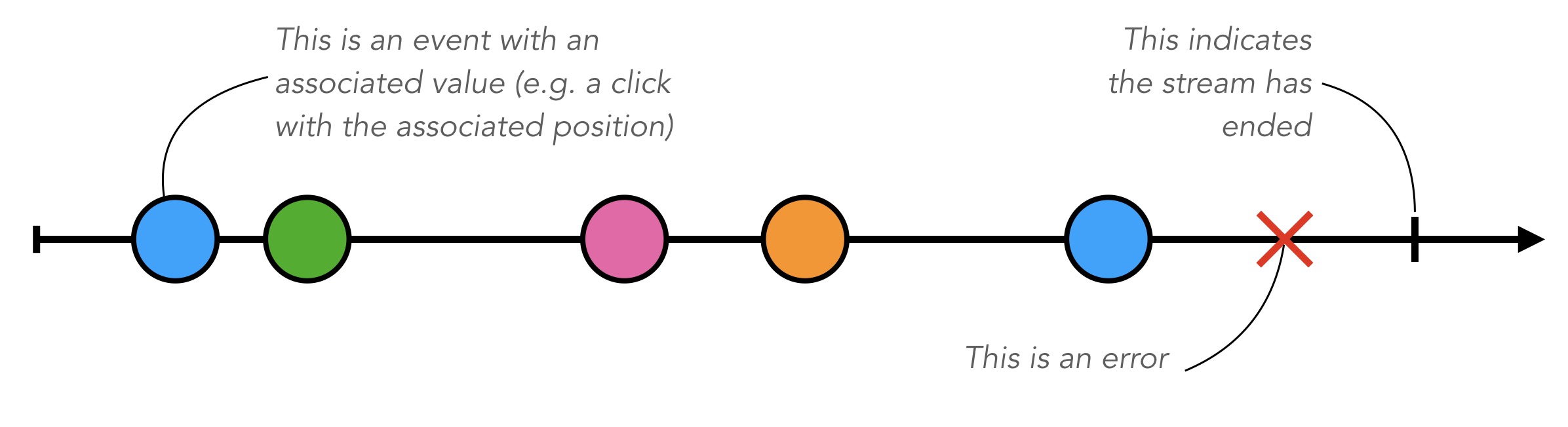
A stream is sequence of ongoing events ordered in time. Streams can be finite or infinite. A Stream's event can be a value, an error or an end signal that indicates the streams has ended.

Coda heavily relies on a reactive programming library called most (see https://mostcore.readthedocs.io/). Coda exposes and extends most with additional data sources (mostly specific sensors), operators (oriented towards motion signal processing) and sinks (graphical operators).

# Creating, Transforming and Consuming Streams

Several Coda operators are "Sources", meaning that they allow you to create data streams. For example, coda provides the periodic source from most, which creates an infinite stream of events that are fired periodically at a fixed period.

To create a periodic stream of period 1 second, we just need to execute the following:

const a = coda.periodic(1000);

However, we have defined the stream but it is not yet runnning. For this, we need to explicitly ask coda to run the stream with a given scheduler (this is only exposing the methods from @most/core):

const a = coda.periodic(1000);
coda.runEffects(a, coda.newDefaultScheduler());

// Create a periodic stream of period 1 second
const a = periodic(1000);

When running the above example, nothing happens: we have created a stream, but it is not consumed anywhere. We need to create a sink that will observe the events happening on the stream and react accordingly.

For example, we can use the standard method tap that will perform side-effects for each event on the stream. We just need to pass a function to tap that does something whenever an event occurs on the stream. For example, we can log the event value directly to the console (note that in the sandbox we can use log instead of console.log).

// Create a periodic stream of period 1 second and log each event to the console
a = periodic(1000).tap(eventValue => {
  log('Received event: ', eventValue);
});

The stream is running because the message 'Received event:' appears in the code example's console. However, periodic creates a stream of undefined events which are not displayed in the console. We can transform the stream to display something more meaningful.

For example, we can successively use the constant and accum operators. constant transform each incoming event into a given value, and accum accumulates numerical values indefinitely.

// Create a periodic stream of period 1 second and log each event to the console
a = periodic(1000)
  .constant(1)
  .accum()
  .tap(x => {
    log('Number of events: ', x);
  });

# Working with User Interactions

In the previous example, we have generated artificial data streams. Coda provides a number of sources that allow you to capture and process user interactions. In this section, we will demonstrate how to manipulate and display a stream of mouse movements.

Wrapping @most/dom-event, Coda provides an easy way to create streams from DOM events. For example, we can capture mouse movements on the entire page using the mousemove operator.

m = mousemove(doc)
  .tap(coords => {
    log(`Mouse coordinates: [${coords}]`);
  });

Coda's mousemove operator creates a stream where an event occurs whenever a mouse movement is detected on the page. Each event's value is an array representing the normalized [x, y] position of the mouse in the given container.

All pointer events produce the same type of stream of coordinates. It is also possible to restrain it to a given HTML element, such as the following box (here, with the click source):

m = click(doc.querySelector('#my-box'))
  .tap(coords => {
    log(`Mouse coordinates: [${coords}]`);
  });

Coda also provides a number of bindings to commercial motion sensing devices (see documentation):

• devicemotion to capture smartphone's motion data
• leapmotion to capture a hand's skeleton with the Leap Motion controller
• myo to capture inertial and EMG data from the Myo Armband
• ...

# Visualizing Data

Coda provides some 'sinks' that allow for the visualization of continuous data streams. The following example displays a basic visualization of the mousemove stream using a plot operator.

m = mousemove(doc)
  .plot({
    legend: 'Mouse position (normalized)',
  });

# Processing Data

Coda provides a number of low-level signal processing operators that are useful to build feature extraction pipelines. This section describes how to compute the overall velocity of the mouse pointer from a stream of mouse positions.

To compute the velocity, we need to differentiate the mousemove position stream. Because events in the mousemove stream only arise when the pointer moves, the stream is not regularly sampled and it is not possible to get a good estimate of the velocity.

We can easily resample the mousemove stream at a fixed sampling rate using the resample operator that takes as argument a second data stream that will "sample" the first one. Here, we will resample the mouse stream at 50 Hz using a periodic stream with 20 ms period:

m = mousemove(doc)
  .plot({
    legend: 'Mouse position (normalized)',
  })
  .resample(periodic(20))
  .plot({
    legend: 'Mouse position (normalized and resampled)',
  });

Because sensor signals can be noisy, we can smooth the signal using a filter, for instance using a moving average filter that smoothes the incoming signal over a window of fixed size (a large window means a lower cutoff frequency).

m = mousemove(doc)
  .resample(periodic(20))
  .plot({
    legend: 'Mouse position (normalized and resampled)',
  })
  .mvavrg({ size: 10 })
  .plot({
    legend: 'Mouse position (normalized, resampled and smoothed)',
  })
  .mvavrg({ size: 40 })
  .plot({
    legend: 'Mouse position (normalized, resampled and VERY smoothed)',
  });

Now the the signal is regularly sampled and smooth, we can differentiate it to obtain the XY velocity of the pointer.

m = mousemove(doc)
  .resample(periodic(20))
  .mvavrg({ size: 10 })
  .plot({
    legend: 'Mouse position (normalized, resampled and smoothed)',
  })
  .delta({ size: 5 })
  .plot({
    legend: 'Mouse velocity',
  });

Finally, we can take the norm of the velocity signal so obtain the absolute velocity of the pointer.

m = mousemove(doc)
  .resample(periodic(20))
  .mvavrg({ size: 10 })
  .delta({ size: 5 })
  .plot({
    legend: 'Mouse velocity (x, y)',
  })
  .norm()
  .plot({
    legend: 'Overall Mouse velocity',
  });

That's it!

This example illustrates how reactive programming can provide a compact and intuitive syntax for building feature extraction pipeliens in minutes.

For more signal processing operators, check out the documentation of the core library.